Thursday, September 28, 2017

Physical Cameras in Stingray

This is a quick blog to share some of the progress Olivier Dionne and I made lately with Physical Cameras in Stingray. Our goal of implementing a solid physically based pipeline has always been split in three phases. First we validated our standard material. We then added physical lights. And now we are wrapping it up with a physical camera.

We define a physical camera as an entity controlled by the same parameters a real world camera would use. These parameters are split into two groups which corresponds to the two main parts of a camera. The camera body is defined by it's sensor size, iso sensitivity, and a range of available shutter speeds. The camera lens is defined by it's focal length, focus range, and range of aperture diameters. Setting all of these parameters should expose the incoming light the same way a real world camera would.

Stingray Representation

Just like our physical light, our camera is expressed as an entity with a bunch of components. The main two components being the Camera Body and the Camera Lens. We then have a transform component and a camera component which together represents the view projection matrix of the camera. After that we have a list of shading environment components which we deem relevant to be controlled by a physical camera (all post effects relevent to a camera). The state of these shading environment components is controled through a script component called the "Physical Camera Properties Mapper" (more on this later). Here is a glimpse of what the Physical Camera entity may look like (wip):

So while there are a lot of components that belongs to a physical camera, the user is expected to interact mainly with the body and the lens components.

Post Effects

A lot of our post effects are dedicated to simulate some sort of camera/lens artifact (DOF, motion blur, film grain, vignetting, bloom, chromatic aberation, ect). One thing we wanted was the ability for physical cameras to override the post processes defined in our global shading environments. We also wanted to let users easily opt out of the physically based mapping that occurred between a camera and it's corresponding post-effect. For example a physical camera will generate an accurate circle of confusion for the depth of field effect, but a user might be frustrated by the limitations imposed by a physically correct dof effect. In this case a user can opt out by simply deleting the "Depth Of Field" component from the camera entity.

It's nice to see how the expressiveness of the Stingray entity system is shaping up and how it enables us to build these complex entities without the need to change much of the engine.

Properties Mapper

All of the mapping occurs in the properties mapper component which I mentioned earlier. This is simply a lua script that gets executed whenever any of the entity properties are edited.

The most important property we wanted to map was the exposure value. We wanted the f-stop, shutter speed, and ISO values to map to an exposure value which would simulate how a real camera sensor reacts to incoming light. Lucky for us this topic is very well covered by Sebastien Lagarde and Charles de Rousiers in their awesome awesome awesome Moving Frostbite to Physically Based Rendering document. The mapping basically boils down to:

local function compute_ev(aperture, shutter_time, iso)
 local ev_100 = log2((aperture * aperture * 100) / (shutter_time * iso))
 local max_luminance = 1.2 * math.pow(2, ev_100)
 return (1 / max_luminance)
end

The second property we were really interested in mapping is the field of view of the camera. Usually the horizontal FOV is calculated as 2 x atan(h/2f) where h is the camera sensor's width and f is the current focal length of the lens. This by itself gives a good approximation of the FOV of a lens, but as was pointed out by the MGS5 & Fox Engine presentation, the focus distance of the lens should also be considered when calculating the FOV from the camera properties.

Intuitively we though that the change in the FOV was caused by a change in the effective focal length of the lens. Adjusting the focus usually shifts a group of lenses up and down the optical axis of a camera lens. Our best guess was that this shift would increase or decrease the effective focal length of the camera lens. Using this idea we we're able to simulate the effect that changing the focus point has on the FOV of a camera:

local function compute_fov(focal_length, film_back_height, focus)
 local normalized_focus = (focus - 0.38)/(5.0 - 0.38)
 local focal_length_offset = lerp(0.0, 1.0, normalized_focus)
 return 2.0 * math.atan(film_back_height/(2.0 * (focal_length + focal_length_offset)))
end

While this gave us plausible results in some cases, it does not map accurately to a real world camera with certain lens settings. For example we can choose a focal length offset that gives good FOV mapping for a zoom lens set to 24mm but incorrect FOV results when it's set to 70mm (see video above). This area of lens optics is one we would like to explore more in the future.

In the future we will map more camera properties to their corresponding post-effects. More on this in a follow up blog.

Validating Results

To validate our mappings we designed a small, controlled environment room that we re-created in stingray. This idea was inspired by the "Conference Room" setup that was presented by Hideo Kojima in the MGS5 & Fox Engine presentation. We used our simplified, environment room to compare our rendered results with real world photographs.

Controlled Environment:

Stingray Equivalent:

Since there is no convenient way to adjust the white balancing in Stingray, we decided to white balance our camera data and use a pure white light in our Stingray scene. We also decided to compare the photos and renders in linear space in the hope to minimize the source of potential error.

White balancing our photographs:

Our very first comparison we're disapointing:

We tracked down the difference in brightness to a problem with how we expressed our light intensity. We discovered that we made the mistake of using the specified lumen value of our lights as it's light intensity. The total luminous flux is expressed in lumens, but the luminous intensity (what the material shader is interested in) is actually the luminous flux per solid angle. So while we let the users enter the "intensity" of lights in lumens, we need to map this value to luminous intensity. The mapping is done as lumens/2π(1-cos(½α)) where α is the apex angle of the light. Lots of details can be found here. This works well for point lights and spot lights. In the future our directional lights will be assumed to be the sun or moon and will be expressed in lux, perhaps with a corresponding disk size.

With this fix in place we started getting more encouraging results:

There is lots left to do but this feels like a very good start to our physically based cameras. This is my last post on the Stingray blog but you can follow Olivier on Twitter if you want to stay up to date with the advances made by the Stingray rendering team. Cheers!

Sunday, July 16, 2017

Validating materials and lights in Stingray

Stingray 1.9 is just around the corner and with it will come our new physical lights. I wanted to write a little bit about the validation process that we went through to increase our confidence in the behaviour of our materials and lights.

Early on we were quite set on building a small controlled "light room" similar to what the Fox Engine team presented at GDC as a validation process. But while this seemed like a fantastic way to confirm the entire pipeline is giving plausible results, it felt like identifying the source of discontinuities when comparing photographs vs renders might involve a lot of guess work. So we decided to delay the validation process through a controlled light room and started thinking about comparing our results with a high quality offline renderer. Since SolidAngle joined Autodesk last year and that we had access to an Arnold license server it seemed like a good candidate. Note that the Arnold SDK is extremely easy to use and can be downloaded for free. If you don't have a license you still have access to all the features and the only limitation is that the rendered frames are watermarked.

We started writing a Stingray plugin that supported simple scene reflection into Arnold. We also implemented a custom Arnold Output Driver which allowed us to forward Arnold's linear data directly into the Stingray viewport where they would be gamma corrected and tonemapped by Stingray (minimizing as many potential sources of error).

Material parameters mapping

The trickiest part of the process was to find an Arnold material which we could use to validate. When we started this work we used Arnold 4.3 and realized early that the Arnold's Standard shader didn't map very well to the Metallic/Roughness model. We had more luck using the alSurface shader with the following mapping:

// "alSurface"
// =====================================================================================
AiNodeSetRGB(surface_shader, "diffuseColor", color.x, color.y, color.z);
AiNodeSetInt(surface_shader, "specular1FresnelMode", 0);
AiNodeSetInt(surface_shader, "specular1Distribution", 1);
AiNodeSetFlt(surface_shader, "specular1Strength", 1.0f - metallic);
AiNodeSetRGB(surface_shader, "specular1Color", white.x, white.y, white.z);
AiNodeSetFlt(surface_shader, "specular1Roughness", roughness);
AiNodeSetFlt(surface_shader, "specular1Ior", 1.5f); // ior = (n-1)^2/(n+1)^2 for 0.04
AiNodeSetRGB(surface_shader, "specular1Reflectivity", white.x, white.y, white.z);
AiNodeSetRGB(surface_shader, "specular1EdgeTint", white.x, white.y, white.z);

AiNodeSetInt(surface_shader, "specular2FresnelMode", 1);
AiNodeSetInt(surface_shader, "specular2Distribution", 1);
AiNodeSetFlt(surface_shader, "specular2Strength", metallic);
AiNodeSetRGB(surface_shader, "specular2Color", color.x, color.y, color.z);
AiNodeSetFlt(surface_shader, "specular2Roughness", roughness);
AiNodeSetRGB(surface_shader, "specular2Reflectivity", white.x, white.y, white.z);
AiNodeSetRGB(surface_shader, "specular2EdgeTint", white.x, white.y, white.z);

Stingray VS Arnold: roughness = 0, metallicness = [0, 1]

Stingray VS Arnold: metallicness = 1, roughness = [0, 1]

Halfway through the validation process Arnold 5.0 got released and with it came the new Standard Surface shader which is based on a Metalness/Roughness workflow. This allowed for a much simpler mapping:

// "aiStandardSurface"
// =====================================================================================
AiNodeSetFlt(standard_shader, "base", 1.f);
AiNodeSetRGB(standard_shader, "base_color", color.x, color.y, color.z);
AiNodeSetFlt(standard_shader, "diffuse_roughness", 0.f); // Use Lambert for diffuse

AiNodeSetFlt(standard_shader, "specular", 1.f);
AiNodeSetFlt(standard_shader, "specular_IOR", 1.5f); // ior = (n-1)^2/(n+1)^2 for 0.04
AiNodeSetRGB(standard_shader, "specular_color", 1, 1, 1);
AiNodeSetFlt(standard_shader, "specular_roughness", roughness);
AiNodeSetFlt(standard_shader, "metalness", metallic);

Investigating material differences

The first thing we noticed is an excess in reflection intensity for reflections with large incident angles. Arnold supports Light Path Expressions which made it very easy to compare and identify the term causing the differences. In this particular case we quickly identified that we had an energy conservation problem. Specifically the contribution from the Fresnel reflections was not removed from the diffuse contribution:

Scenes with a lot of smooth reflective surfaces demonstrates the impact of this issue noticeably:

Another source of differences and confusion came from the tint of the Fresnel term for metallic surfaces. Different shaders I investigaed had different behaviors. Some tinted the Fresnel term with the base color while some others didn't:

It wasn't clear to me how Fresnel's law of reflection applied to metals. I asked on Twitter what peoples thoughts were on this and got this simple and elegant claim made by Brooke Hodgman: "Metalic reflections are coloured because their Fresnel is wavelength varying, but Fresnel still goes to 1 at 90deg for every wavelength". This convinced me instantly that indeed the correct thing to do was to use an un-tinted Fresnel contribution regardless of the metallicness of the material. I later found this graph which also confirmed this:

For the Fresnel term we use a pre filtered Fresnel offset stored in a 2d lut (as proposed by Brian Karis in Real Shading in Unreal Engine 4). While results can diverge slightly from Arnold's Standard Surface Shader (see "the effect of metalness" from Zap Anderson's Physical Material Whitepaper), in most cases we get an edge tint that is pretty close:

Investigating light differences

With the brdf validated we could start looking into validating our physical lights. Stingray currently supports point, spot, and directional lights (with more to come). The main problem we discovered with our lights is that the attenuation function we use is a bit awkward. Specifically we attenuate by I/(d+1)^2 as opposed to I/d^2 (Where 'I' is the intensity of the light source and 'd' is the distance to the light source from the shaded point). The main reason behind this decision is to manage the overflow that could occur in the light accumulation buffer. Adding the +1 effectively clamps the maximum value intensity of the light as the intensity set for that light itself i.e. as 'd' approaches zero 'I' approaches the intensity set for that light (as opposed to infinity). Unfortunatly this decision also means we can't get physically correct light falloffs in a scene:

Even if we scale the intensity of the light to match the intensity for a certain distance (say 1m) we still have a different falloff curve than the physically correct attenuation. It's not too bad in a game context, but in the architectural world this is a bigger issue:

This issue will be fixed in Stingray 1.10. Using I/(d+e)^2 (where 'e' is 1/max_value along) with an EV shift up and down while writing and reading from the accumulation buffer as described by Nathan Reed is a good step forward.

Finally we were also able to validate our ies profile parser/shader and our color temperatures behaved as expected:

Results and final thoughts

Integrating a high quality offline renderer like Arnold has proven invaluable in the process of validating our lights in Stingray. A similar validation process could be applicable to many other aspects of our rendering pipeline (antialiasing, refractive materials, fur, hair, post-effects, volumetrics, ect)

I also think that it can be a very powerful tool for content creators to build intuition on the impact of indirect lighting in a particular scene. For example in a simple level like this, adding a diffuse plane dramatically changes the lighting on the Buddha statue:

The next step is now to compare our results with photographs gathered from a controlled environments. To be continued...


Monday, July 3, 2017

Physically Based Lens Flare

While playing Horizon Zero Dawn I got inspired by the lens flare they supported and decided to look into implementing some basic ones in Stingray. There were four types of flare I was particularly interested in.
  1. Anisomorphic flare
  2. Aperture diffraction (Starbursts)
  3. Camera ghosts due to Sun or Moon (High Quality - What this post will cover)
  4. Camera ghosts due to all other light sources (Low Quality - Screen Space Effect)
Image credits: Die Hard (1), Just Another Dang Blog (2), PEXELS (3), The Matrix Reloaded (4)

Once finished I'll do a follow up blog post on the Camera Lens Flare plugin, but for now I want to share the implementation details of the high-quality ghosts which are an implementation of "Physically-Based Real-Time Lens Flare Rendering".

Code and Results

All the code used to generate the images and videos of this article can can be found on github.com/greje656/PhysicallyBasedLensFlare.


Ghosts

The basic idea of the "Physically-Based Lens Flare" paper is to ray trace "bundles" into a lens system which will end up on a sensor to form a ghost. A ghost here refers to the de-focused light that reaches the sensor of a camera due to the light reflecting off the lenses. Since a camera lens is not typically made of a single optical lens but many lenses there can be many ghosts that form on it's sensor. If we only consider the ghosts that are formed from two bounces, that's a total of nCr(n,2) possible ghosts combinations (where n is the number of lens components in a camera lens)


Lens Interface Description

Ok let's get into it. To trace rays in an optical system we obviously need to build an optical system first. This part can be tedious. Not only have you got to find the "Lens Prescription" you are looking for, you also need to manually parse it. For example parsing the Nikon 28-75mm patent data might look something like this:


There is no standard way of describing such systems. You may find all the information you need from a lens patent, but often (especially for older lenses) you end up staring at an old document that seems to be missing important information required for the algorithm. For example, the Russian lens MIR-1 apparently produces beautiful lens flare, but the only lens description I could find for it was this:

MIP.1B manual

Ray Tracing

Once you have parsed your lens description into something your trace algorithm can consume, you can then start to ray trace. The idea is to initialize a tessellated patch at the camera's light entry point and trace through each of the points in the direction of the incoming light. There are a couple of subtleties to note regarding the tracing algorithm.

First, when a ray misses a lens component the raytracing routine isn't necessarily stopped. Instead if the ray can continue with a path that is meaningful the ray trace continues until it reaches the sensor. Only if the ray misses the sphere formed by the radius of the lens do we break the raytracing routine. The idea behind this is to get as many traced points to reach the sensor so that the interpolated data can remain as continuous as possible. Rays track the maximum relative distance it had with a lens component while tracing through the interface. This relative distance will be used in the pixel shader later to determine if a ray had left the interface.

Relative distance visualized as green/orange gradient (black means ray missed lens component completely)

Secondly, a ray bundle carries a fixed amount of energy so it is important to consider the distortion of the bundle area that occurs while tracing them. In In the paper, the author states:
"At each vertex, we store the average value of its surrounding neighbours. The regular grid of rays, combined with the transform feedback (or the stream-out) mechanism of modern graphics hardware, makes this lookup of neighbouring quad values very easy"
I don't understand how the transform feedback, along with the available adjacency information of the geometry shader could be enough to provide the information of the four surrounding quads of a vertex (if you know please leave a comment). Luckily we now have compute and UAVs which turn this problem into a fairly trivial one. Currently I only calculate an approximation of the surrounding areas by assuming the neighbouring quads are roughly parallelograms. I estimate their bases and heights as the average lengths of their top/bottom, left/right segments. The results are seen as caustics forming on the sensor where some bundles converge into tighter area patches while some other dilates:


This works fairly well but is expensive. Something that I intend to improve in the future.

Now that we have a traced patch we need to make some sense out of it. The patch "as is" can look intimidating at first. Due to early exits of some rays the final vertices can sometimes look like something went terribly wrong. Here is a particularly distorted ghost:


The first thing to do is discard pixels that exited the lens system:
float intensity1 = max_relative_distance < 1.0f;
float intensity = intensity1;
if(intensity == 0.f) discard;

Then we can discard the rays that didn't have any energy as they entered to begin with (say outside the sun disk):
float lens_distance = length(entry_coordinates.xy);
float sun_disk = 1 - saturate((lens_distance - 1.f + fade)/fade);
sun_disk = smoothstep(0, 1, sun_disk);
//...
float intensity2 = sun_disk;
float intensity = intensity1 * intensity2;
if(intensity == 0.f) discard;

Then we can discard the rays that we're blocked by the aperture:
//...
float intensity3 = aperture_sample;
float intensity = intensity1 * intensity2 * intensity3;
if(intensity == 0.f) discard;

Finally we adjust the radiance of the beams based on their final areas:
//...
float intensity4 = (original_area/(new_area + eps)) * energy;
float intensity = intensity1 * intensity2 * intensity3 * intensity4;
if(intensity == 0.f) discard;

The final value is the rgb reflectance value of the ghost modulated by the incoming light color:
float3 color = intensity * reflectance.xyz * TempToColor(INCOMING_LIGHT_TEMP);

Aperture


Image credits: 6iee

The aperture shape is built procedurally. As suggested by Padraic Hennessy's blog I use a signed distance field confined by "n" segments and threshold it against some distance value. I also experimented with approximating the light diffraction that occurs at the edge of the apperture blades using a simple function:


Finally, I offset the signed distance field with a repeating sin function which can give curved aperture blades:


Starburst

The starburst phenomena is due to light diffraction that passes through the small aperture hole. It's a phenomena known as the "single slit diffraction of light". The author got really convincing results to simulate this using the Fraunhofer approximation. The challenge with this approach is that it requires bringing the aperture texture into Fourier space which is not trivial. In previous projects I used Cuda's math library to perform the FFT of a signal but since the goal is to bring this into Stingray I didn't want to have such a dependency. Luckily I found this little gem posted by Joseph S. from intel. He provides a clean and elegant compute implementation of the butterfly passes method which bring a signal to and from Fourier space. Using it I can feed in the aperture shape and extract the Fourier Power Spectrum:


This spectrum needs to be filtered further in order to look like a starburst. This is where the Fraunhofer approximation comes in. The idea is to basically reconstruct the diffraction of white light by summing up the diffraction of multiple wavelengths. The key observation is that the same Fourier signal can be used for all wavelengths. The only thing needed is to scale the sampling coordinates of the Fourier power spectrum:

(x0,y0) = (u,v)·λ·z0 for λ = 350nm/435nm/525nm/700nm

Summing up the wavelengths gives the starburst image. To get more interesting results I apply an extra filtering step. I use a spiral pattern mixed with a small rotation to get rid of any left over radial ringing artifacts (judging by the author's starburst results I suspect this is a step they are also doing):


Anti Reflection Coating

While some appreciate the artistic aspect of lens flare, lens manufacturers work hard to minimize them by coating lenses with anti-reflection coatings. The coating applied to each lenses are usually designed to minimize the reflection of a specific wavelength. They are defined by their thickness and index of refraction. Given the wavelength to minimize reflections for, and the IORs of the two medium involved in the reflection (say n0 and n2), the ideal IOR (n1) and thickness (d) of the coating are defined as n1 = sqrt(n0·n2) and d=λ/4·n1. This is known as a quarter wavelength anti-reflection coating. I've found this site very helpful to understand this phenomenon.

In the current implementation each lens coating specifies a wavelength the coating should be optimized for and the ideal thickness and IOR are used by default. I added a controllable offset to thicken the AR coating layer in order to conveniently reduce it's anti-reflection properties:

No AR Coating:

Ideal AR Coating:

AR Coating with offsetted thickness:

Optimisations

Currently the full cost of the effect for a Nikon 28-75mm lens is 12ms (3ms to ray march 352x32x32 points and 9ms to draw the 352 patches). The performance degrades as the sun disk is made bigger since it results in more and more overshading during the rasterisation of each ghosts. With a simpler lens interface like the 1955 Angenieux the cost decreases significantly. In the current implementation every possible "two bounce ghost" is traced and drawn. For a lens system like the Nikon 28-75mm which has 27 lens components, that's n!/r!(n-r)! = 352 ghosts. It's easy to see that this number can increase dramatically with the number of component.

An obvious optimization would be to skip ghosts that have intensities so low that their contributions are imperceptible. Using Compute/DrawIndirect it would be fairly simple to first run a coarse pass and use it to cull non contributing ghosts. This would reduce the compute and rasterization pressure on the gpu dramatically. Something I intend to do in future.

Conclusion

I'm not sure if this approach was ever used in a game. It would probably be hard to justify it's heavy cost. I feel this would have a better use case in the context of pre-visualization where a director might be interested in having early feedback on how a certain lens might behave in a shot.

Image credits: Wallup

Image credits: Wallpapers Web

Finally, be aware the author has filled a patent for the algorithm described in his paper, which may put limits on how you may use parts of what is described in my post. Please contact the paper's author for more information on what restrictions might be in place.

Thursday, June 22, 2017

Reprojecting Reflections

Screen space reflections are such a pain. When combined with taa they are even harder to manage. Raytracing against a jittered depth/normal g-buffer can easily cause reflection rays to have widely different intersection points from frame to frame. When using neighborhood clamping, it can become difficult to handle the flickering caused by too much clipping especially for surfaces that have normal maps with high frequency patterns in them.

On top of this, reflections are very hard to reproject. Since they are view dependent simply fetching the motion vector from the current pixel tends to make the reprojection "smudge" under camera motion. Here's a small video grab that I did while playing Uncharted 4 (notice how the reflections trails under camera motion)


Last year I spent some time trying to understand this problem a little bit more. I first drew a ray diagram describing how a reflection could be reprojected in theory. Consider the goal of reprojecting the reflection that occurs at incidence point v0 (see diagram bellow), then to reproject the reflection which occurred at that point you would need to:
  1. Retrieve the surface motion vector (ms) corresponding to the reflection incidence point (v0)
  2. Reproject the incidence point using (ms)
  3. Using the depth buffer history, reconstruct the reflection incidence point (v1)
  4. Retrieve the motion vector (mr) corresponding to the reflected point (p0)
  5. Reproject the reflection point using (mr)
  6. Using the depth buffer history, reconstruct the previous reflection point (p1)
  7. Using the previous view matrix transform, reconstruct the previous surface normal of the incidence point (n1)
  8. Project the camera position (deye) and the reconstructed reflection point (dp1) onto the previous plane (defined by surface normal = n1, and surface point = v1)
  9. Solve for the position of the previous reflection point (r) knowing (deye) and (dp1)
  10. Finally, using the previous view-projection matrix, evaluate (r) in the previous reflection buffer


By adding to Stingray a history depth buffer and using the previous view-projection matrix I was able to confirm this approach could successfully reproject reflections.
float3 proj_point_in_plane(float3 p, float3 v0, float3 n, out float d) {
 d = dot(n, p - v0);
 return p - (n * d);
}

float3 find_reflection_incident_point(float3 p0, float3 p1, float3 v0, float3 n) {
 float d0 = 0;
 float d1 = 0;
 float3 proj_p0 = proj_point_in_plane(p0, v0, n, d0);
 float3 proj_p1 = proj_point_in_plane(p1, v0, n, d1);

 if(d1 < d0)
  return (proj_p0 - proj_p1) * d1/(d0+d1) + proj_p1;
 else
  return (proj_p1 - proj_p0) * d0/(d0+d1) + proj_p0;
}

float2 find_previous_reflection_position(
 float3 ss_pos, float3 ss_ray,
 float2 surface_motion_vector, float2 reflection_motion_vector,
 float3 world_normal) {
 float3 ss_p0 = 0;
 ss_p0.xy = ss_pos.xy - surface_motion_vector;
 ss_p0.z = TEX2D(input_texture5, ss_p0.xy).r;

 float3 ss_p1 = 0;
 ss_p1.xy = ss_ray.xy - reflection_motion_vector;
 ss_p1.z = TEX2D(input_texture5, ss_p1.xy).r;

 float3 view_n = normalize(world_to_prev_view(world_normal, 0));
 float3 view_p0 = float3(0,0,0);
 float3 view_v0 = ss_to_view(ss_p0, 1);
 float3 view_p1 = ss_to_view(ss_p1, 1);

 float3 view_intersection = 
  find_reflection_incident_point(view_p0, view_p1, view_v0, view_n);
 float3 ss_intersection = view_to_ss(view_intersection, 1);

 return ss_intersection.xy;
}

You can see in these videos that most of the reprojection distortion in the reflections are addressed:


Ghosting was definitely minimized under camera motion. The video bellow compares the two reprojection method side by side.

LEFT: Simple Reprojection, RIGHT: Correct Reprojection
(note that I disabled neighborhood clamping in this video to visualize the reprojection better)

So instead I tried a different approach. The new idea was to pick a few reprojection vectors that are likely to be meaningful in the context of a reflection. Originally I looked into:
  • Motion vector at ray incidence
  • Motion vector at ray intersection
  • Parallax corrected motion vector at ray incidence
  • Parallax corrected motion vector at ray intersection

The idea of doing parallax correction on motion vectors for reflections came from the Stochastic Screen-Space Reflections talk presented by Tomasz Stachowiak at Siggraph 2015. Right now here's how it's currently implemented although I'm not 100% sure that's as correct as it could be (there's a PARALLAX_FACTOR define which I needed to manually tweak to get optimal results. Perhaps there's a better way of doing this)?
float2 parallax_velocity = velocity * saturate(1.0 - total_ray_length * PARALLAX_FACTOR);
Once all those interesting vectors are retrieved, the one with the smallest magnitude is declared as "the most likely succesful reprojection vector". This simple idea alone has improved the reprojection of the ssr buffer quite significantly (note that if casting multiple rays per pixel, then averaging the sum of all succesful reprojection vectors still gave us a better reprojection than what we had previously)


Screen space reflections is one of the most difficult screen space effect I've had to deal with. They are plagued with artifacts which can often be difficult to explain or understand. In the last couple of years I've seen people propose really creative ways to minimize some of these artifacts that are inherent to ssr. I hope this continues!

Tuesday, May 16, 2017

Rebuilding the Entity Index

Background

If you are not familiar with the Stingray Entity system you can find good resources to catch up here:
The Entity system is a very central part of the future of Stingray and as we integrate it with more parts new requirements pops up. One of those is the ability to interact with Entity Components via the visual scripting language in Stingray - Flow. We want to provide a generic interface to Entites in Flow without adding weight to the fundamental Entity system.

To accomplish this we added a “Property” system that Flow and other parts of the Stingray Engine can use which is optional for each Component to implement in addition to having its own specialized API. The Property System enables an API to read and write entity component properties using the name of component, the property name and the property value. The Property System needs to be able to find a specific Component Instance by name for an Entity, and the Entity System does not directly track an Entity / Component Instance relationship. It does not even track the Entity / Component Manager relationship.

So what we did was to add the Entity Index, a registry where we add all Component Instances created for an Entity as it is constructed from an Entity Resource. To make it usable we also added the rule that each Component in an Entity Resource should have a unique name within the resource so the user can identify it by name when using the Flow system.

In order for the Flow system to work we need to be able to find a specific component instance by name for an Entity so we could get and set properties of that instance. This is the job of the Entity Index. In the Entity Index you can register an Entitys components by name so you later can do a lookup.

Property System and Entity Index

When creating an Entity we use the name of the component instance together with the component type name, i.e the Component Manager, and create an Entity Index that maps the name to the component instance and the Component Manager. In the Stingray Entity system an Entity cannot have two component instances with the same name.

Example:


Entity

  • Transform - Transform Component
  • Fog - Render Data Component
  • Vignette - Render Data Component

For this Entity we would instantiate one Transform Component Instance and two Render Data Component Instances. We get back an InstanceId for each Component Instance which can be used to identify which of Fog or Vignette we are talking about even though they are created from the same Entity using the same Component Manager.

We also register this in the Entity Index as:

Key Value
Entity Array<Components>

The Array<Components> contains one or more entries which each contain the following:

Components
Component Manager
InstanceId
Name

Lets add the a few entities and components to the Entity Index:

entity_1.id

Name Component Manager InstanceId
hash(“Transform”) &transform_manager 13
hash(“Fog”) &render_data_manager_1 4
hash(“Vignette”) &render_data_manager_1 5


entity_2.id

Name Component Manager InstanceId
hash(“Transform”) &transform_manager 14
hash(“Fog”) &render_data_manager_1 6
hash(“Vignette”) &render_data_manager_1 7


entity_3.id

Name Component Manager InstanceId
hash(“Transform”) &transform_manager 2
hash(“Fog”) &render_data_manager_2 4
hash(“Vignette”) &render_data_manager_2 5

This allows Flow to set and get properties using the Entity and the Component Name. Using the Entity and Component Name we can look up which Component Manager has the component instance and which InstanceId it has assigned to it so we can get the Instance and operate on the data.

The problem with this implementation is that it will become very large - we need a large registry with one key-array pair for each Entity where the array contains one entry for each Component Instance for the Entity, not very efficient as the number of entites grow. There is no reuse at all in the Entity Index - and it can’t be - each entry in the index is unique with no overlap.

Here are some measurements using a synthetic test that creates entities, add and looks up components on the entities and deleted entities. It deletes parts of the entities as it runs and does garbage collection. The number entities given in the tables is the total number created during the test, not the number of simultaneous entities which varies over time. The entities has 75 different types of component compositions, ranging from a single component to eleven for other entities. The test is single threaded and no locking besides some on the memory sub system which makes the times match up well with CPU usage.

Entity Count Test run time (s) Memory used (Mb) Time/Entity (us)
10k 0.01 5.79 0.977
20k 0.01 5.79 0.488
40k 0.03 11.88 0.732
80k 0.06 11.88 0.732
160k 0.13 25.69 0.793
320k 0.32 31.04 0.977
640k 1.08 55.90 1.648
1.28m 2.58 65.82 1.922
2.56m 6.35 65.55 2.366
5.12m 13.42 120.55 2.500
10.24m 25.69 130.55 2.393

As you can see we start to take longer and longer time and use more and more memory as we double the number of entities and as we get to the larger numbers the time and memory increases pretty dramatically.


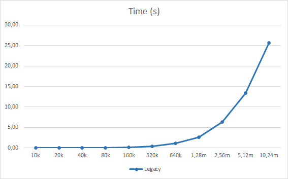
Since we plan to use the entity system extensively we need an index that is more efficient with memory and scales more linearly in CPU usage.

Shifting control of the InstanceId

The InstanceId is defined to be unique to the Entity instance for a specific Component Manager - it does not have to be unique for all components in a Component Manager, nor does it have to be unique across different Component Managers.

The create and lookup functions for an Component Instance looks like this:

InstanceWithId instance_with_id = transform_manager.create(entity);
InstanceId my_transform_id = instance_with_id.id;

.....

Instance instance = transform_manager.lookup(entity, my_transform_id);

The interface is somewhat confusing since the create function returns both the component instance id and the instance. This is done so you don’t have to do a lookup of the instance directly after create. As you can see we have no knowledge of what the resulting InstanceId will be so we can’t make any assumptions in the Entity Index forcing us to have unique entries for each Component instance of every Entity.

But we already set up the rule that in the Entity Resource, each Component should have a unique name for the Property System to work - this is a new requirement that was added at a later stage than when designing the initial Entity system. Now that it is there we can make use of this to simplify the Entity Index.

Instead of letting each Component Manager decide the InstanceId we let the caller to the create function decide the InstanceId. We can decide that the InstanceId should be the 32-bit hash of the Component Name from the Entity Resource. Doing this will restrict the possible optimization that a component manager could do if it had control of the InstanceId, but so far we have had no real use case for it and the benefits of changing this are greater than the loss of a possible optimization that we might do sometime in the future.

So we change the API like this:

Instance instance = transform_manager.create(entity, hash("Transform"));

.....

Instance instance = transform_manager.lookup(entity, hash("Transform")); 

Nice, clean and symmetrical. Note though that the InstanceId is entierly up to the caller to control, it does not have to be a hash of a string. It must be unique for an Entity within a specific component manager. Having it work with the Entity Index and the Property System the InstanceId needs to be unique across all Component Instances in all Component Managers for each Entity instance. This is enforced when an Entity is created from a resource but not when constructing Component Instances by hand in code. If you want a component added outside the resource construction to work with the Property System care needs to be taken so it does not collide with other names of component instances for the Entity.

Lets add the entities and components again using the new rule set, the Entity Index now look like this:

entity_1.id

Name Component Manager InstanceId
hash(“Transform”) &transform_manager hash(“Transform”)
hash(“Fog”) &render_data_manager_1 hash(“Fog”)
hash(“Vignette”) &render_data_manager_1 hash(“Vignette”)


entity_2.id

Name Component Manager InstanceId
hash(“Transform”) &transform_manager hash(“Transform”)
hash(“Fog”) &render_data_manager_1 hash(“Fog”)
hash(“Vignette”) &render_data_manager_1 hash(“Vignette”)


entity_3.id

Name Component Manager InstanceId
hash(“Transform”) &transform_manager hash(“Transform”)
hash(“Fog”) &render_data_manager_2 hash(“Fog”)
hash(“Vignette”) &render_data_manager_2 hash(“Vignette”)

As we now see the Instance Id column now contain redundant data - we only need to store the Component Manager pointer. We use the Entity and hash the component name to find our Component Manager which can be used to look up the Instance.

entity_1.id

Name Component Manager
hash(“Transform”) &transform_manager
hash(“Fog”) &render_data_manager_1
hash(“Vignette”) &render_data_manager_1


entity_2.id

Name Component Manager
hash(“Transform”) &transform_manager
hash(“Fog”) &render_data_manager_1
hash(“Vignette”) &render_data_manager_1


entity_3.id

Name Component Manager
hash(“Transform”) &transform_manager
hash(“Fog”) &render_data_manager_2
hash(“Vignette”) &render_data_manager_2


We now also see that the lookup array for entity_1 and entity_2 are identical so two keys could point to the same value.

Options for implementation

We could opt for an index that has a map from entity_id to a list or map of entries for lookup:

entity_1.id = [ hash("Transform"), &transform_manager ], [ hash("Fog"), &render_data_manager_1 ], [ hash("Vignette"), &render_data_manager_1 ]
entity_2.id = [ hash("Transform"), &transform_manager ], [ hash("Fog"), &render_data_manager_1 ], [ hash("Vignette"), &render_data_manager_1 ]
entity_3.id = [ hash("Transform"), &transform_manager ], [ hash("Fog"), &render_data_manager_2 ], [ hash("Vignette"), &render_data_manager_2 ]

We should probably not store the same entry lookup list multiple times if it can be resused by multiple entity instances as this wastes space, but at any time a new component instance can be added or removed from an entity and its entry list would then change - that would mean administrating memory for the lookup lists and detecting when two entities starts to diverge so we can make a new extended copy of the entry list for the changed entity. We should probably also remove lookup lists that are no longer used as it would waste memory.

Entity and component creation

The call sequence for creating entities from resources (or even programmatically) looks something like this:

Entity e = create();
Instance transform = transform_manager.create(e, hash("Transform"));
Instance fog = render_data_manager_1.create(e, hash("Fog"));
Instance vignette = render_data_manager_1.create(e, hash("Vignette"));

In this scenario we could potentially build a entity lookup list for the entity which contains lookup for the transform, fog and vignette instances:

entity_index.register(e, [ hash("Transform"), &transform_manager ], [ hash("Fog"), &render_data_manager_1 ], [ hash("Vignette"), &render_data_manager_1 ]);

But as stated previously - component instances can be added and removed at any point in time making the lookup table change during the lifetime of the Entity. We need to be able to extend it at will, so it should look something like this:

Entity e = create();
Instance transform = transform_manager.create(e, hash("Transform"));
entity_index.register(e, [ hash("Transform"), &transform_manager ]);

Instance fog = render_data_manager_1.create(e, hash("Fog"));
entity_index.register(e, [ hash("Fog"), &render_data_manager_1 ]);

Instance vignette = render_data_manager_1.create(e, hash("Vignette"));
entity_index.register(e, [ hash("Vignette"), &render_data_manager_1 ]);

Now we just extend the lookup list of the entity as we add new components. This means that two entities that started out life as having identical lookup lists after being spawned from a resource might diverge over time so the Entity Index needs to handle that.

Component Instances can also be destroyed, so we should handle that as well. Even if we do not remove component instances things will still work - if we keep a lookup to an Instance that has been removed we would then just fail the lookup in the corresponding Component Manager. It would lead to waste of memory though, something we need to be aware of going forward.

Building a Prototype chain

Looking at how we build up the Component instances for an Entity it goes something like this: first add the Transform, then add Fog and finally Vignette. This looks sort of like an inheritance chain…
Lets call a lookup list that contains a specific set of entry values a Prototype.

An entity starts with an empty lookup list that contains nothing [], this is the base Prototype, lets call that P0.
  • Add the “Transform” component and your prototype is now P0 + [&transform_manager, “Transform”], lets call that prototype P1.
  • Add the “Fog” component, now the prototype is P1 + [&render_data_manager_1, “Fog”] - call it P2.
  • Add the “Vignette” component, now the prototype is P2 + [&render_data_manager_1, “Vignette”] - call it P3.
Your entity is now using the prototype P3, and from that you can find all the lookup entries you need.
The prototype registry will contain:

P0 = []
P1 = [] + [&transform_manager, "Transform"]
P2 = [] + [&transform_manager, "Transform"] + [&render_data_manager_1, "Fog"]
P3 = [] + [&transform_manager, "Transform"] + [&render_data_manager_1, "Fog"] + [&render_data_manager_1, "Vignette"]

If you create another entity which uses the same Components with the same names you will end up with the same prototype:

Create entity_2, it will have the empty prototype P0.
  • Add the “Transform” component and your prototype now P1.
  • Add the “Fog” component, now the prototype is P2.
  • Add the “Vignette” component, now the prototype is P3.

We end up with the same prototype P3 as the other entity - as long as we add the entities in the same order we end up with the same prototype. For entites created from resources this will be true for all entities created from the same entity resource. For components that are added programatically it will only work if the code adds components in the same order, but even if they do not always do this we still will have a very large overlap for most of the entities.

Lets look at the third example where we do not have an exact match, entity_3:

Create entity_3, it will have the empty prototype P0.
  • Add the “Transform” component and your prototype is now P0 + [&transform_manager:Transform, “Transform”] = P1.
  • Add the “Fog” component - this render data component manager is not the same as entity_1 and entity_2 so we get P1 + [&render_data_manager_2, “Fog”], this does not match P2 so we make a new prototype P4 instead.
  • Add the “Vignette” component, now the prototype is P4 + [&render_data_manager_2, “Vignette”] -> P5.
The prototype registry will contain:

P0 = []
P1 = [] + [&transform_manager, "Transform"]
P2 = [] + [&transform_manager, "Transform"] + [&render_data_manager_1, "Fog"]
P3 = [] + [&transform_manager, "Transform"] + [&render_data_manager_1, "Fog"] + [&render_data_manager_1, "Vignette"]
P4 = [] + [&transform_manager, "Transform"] + [&render_data_manager_2, "Fog"]
P5 = [] + [&transform_manager, "Transform"] + [&render_data_manager_2, "Fog"] + [&render_data_manager_2, "Vignette"]

Storage of the prototype

We can either for each prototype store all the component lookup entries - this makes it easy to get all the component instance look-ups in one go at the expense of memory due to data duplication. Each entity will store which prototype it uses.
  • entity_1 -> P3
  • entity_2 -> P3
  • entity_3 -> P5
The prototype registry now contains:

P0 = []
P1 = [] + [&transform_manager, "Transform"]
P2 = [] + [&transform_manager, "Transform"] + [&render_data_manager_1, "Fog"]
P3 = [] + [&transform_manager, "Transform"] + [&render_data_manager_1, "Fog"] + [&render_data_manager_1, "Vignette"]
P4 = [] + [&transform_manager, "Transform"] + [&render_data_manager_2, "Fog"]
P5 = [] + [&transform_manager, "Transform"] + [&render_data_manager_2, "Fog"] + [&render_data_manager_2, "Vignette"]

Some of the entries (P2 and P4) could technically be removed since they are not actively used - we would need to temporarily re-create them as new entries with the same structure were added.
A different option is to actually use the intermediate entries by referencing them, like so:

P0 = []
P1 = P0 + [&transform_manager, "Transform"]
P2 = P1 + [&render_data_manager_1, "Fog"]
P3 = P2 + [&render_data_manager_1, "Vignette"]
P4 = P1 + [&render_data_manager_2, "Fog"]
P5 = P4 + [&render_data_manager_2, "Vignette"]

Less wasteful but requires lookup up in the chain to find all the components for an entity. On the other hand we can make this very efficient storage-wise by having a lookup table like this:
Map from Prototype to {base_prototype, component_manager, component_name}. The prototype data is small and has no dynamic size so they can be stored very effiently.

The prototype will add all the prototypes to the same prototype map and since the HashMap implementation lookup gives us O(1) lookup cost, traversing the chain will only cost us the potential cache-misses of the lookup. Since the hashmap is likely to be pretty compact (via prototype reuse) this hopefully should not be a huge issue. If it turns out to be, a different storage approach might be needed trading memory use for lookup speed.

Since the amount of data we store for each Prototype would be very small - roughly 16 bytes - we can be a bit more relaxed with unused prototypes - we do not need to remove them as aggressively as we would if each prototype contained a complete lookup table for all components.

Building the Prototype index

So how do we “name” the prototypes effectively for fast lookup? Well, the first lookup would be Entity -> Prototype and then from Prototype -> Prototype definition.
A simple approach would be hashing - use the content of the Prototype as the hash data to get a unique identifier.

The first base prototype has an empty definition so we let that be zero.
To calculate a prototype, mix the prototype you are basing it of with the hash of the protoype data, in our case we hash the Component Manager pointer and Component Name, and mix it with the base prototype.

Prototype prototype = mix(base_prototype, mix(hash(&component_manager), hash(component_name)))

The entry is stored with the prototype as key and the value as [base_prototype, &component_manager, component_name].

When you add a new Component to an entity we add/find the new prototype and update the Entity -> Prototype map to match the new prototype.

So, we end up with a structure like this:
struct PrototypeDescription {
    Prototype base_prototype;
    ComponentMananger *component_manager;
    IdString32 component_name;
}

Map<Entity, Prototype> entity_prototype_lookup;
Map<Prototype, PrototypeDescription> prototypes;

void register_component(Entity, ComponentManager, component_name)
{
    Prototype p = entity_prototype_lookup[Entity];
    Prototype new_p = mix(p, mix(hash(ComponentManager), hash(component_name)));
    if (!prototypes.has(new_p))
        prototypes.insert(new_p, {p, &ComponentManager, component_name});
    enity_index[Entity] = new_p;
}

ComponentMananger *find_component_manager(Entity, component_name)
{
    Prototype p = entity_index[Entity];
    while (p != 0)
    {
        PrototypeDescription description = prototypes[p];
        if (description.component_name == component_name)
            return description.component_manager;
        p = description.base_prototype;
    }
    return nullptr;
}

This could lead to a lot of hashing and look-ups but we can change the api to register new components to multiple Entities in one go which would lead to dramatically less number of hashing and look-ups, we already do that kind of optimization when creating entities from resources so it would be a natural fit. Also, we can easily cache the base prototype index to avoid more of the hash look-ups in find_component_manager.

Measuring the results

Lets run the synthetic test again and see how our new entity index match up to the old one.

Entity Count Test run time (s) Memory used (Mb) Time/Entity (us)
10k 0.01 0.26 0.977
20k 0.01 0.51 0.488
40k 0.03 0.99 0.832
80k 0.06 0.99 0.610
160k 0.11 0.99 0.671
320k 0.23 0.99 0.702
640k 0.46 0.99 0.702
1.28m 0.94 0.99 0.700
2.56m 1.88 0.99 0.700
5.12m 3.78 0.99 0.704
10.24m 7.57 0.99 0.705

The run time now scales very close to linearly and is overall faster than the old implementation. Most notable is the win when using a lot of entities. Memory usage has gone down as well and the time/entity is also scaling more gracefully.


Memory usage looks a little strange but there is an easy explanation - the mapping from entity to prototype is using almost all that memory (via a hashmap) and the actual prototypes takes less than 30 Kb. Note that the old index uses the same amount of memory for the Entity to Prototype mapping.

Lets compare the graphs between the old and new implementation:


Entity Count Time New (s) Time Legacy (s) Memory New (Mb) Memory Legacy (Mb) Time/Entity New (us) Time/Entity Legacy (us)
10k 0.01 0.01 0.26 5.79 0.977 0.977
20k 0.01 0.01 0.51 5.79 0.488 0.488
40k 0.03 0.03 0.99 11.88 0.832 0.732
80k 0.05 0.06 0.99 11.88 0.610 0.732
160k 0.11 0.13 0.99 25.69 0.671 0.793
320k 0.23 0.32 0.99 31.04 0.702 0.977
640k 0.46 1.08 0.99 55.90 0.702 1.648
1.28m 0.94 2.58 0.99 65.82 0.700 1.922
2.56m 1.88 6.53 0.99 65.55 0.700 2.366
5.12m 3.78 13.42 0.99 120.55 0.704 2.500
10.24m 7.57 25.69 0.99 130.55 0.705 2.393


Looks like a pretty good win.

Final words

By taking into account the new requirements as the Entity system evolved we were able to create a much more space efficient and more performant Entity Index.

The implementation chosen here has focused on reducing the amount of data we use in the Entity Index at the cost of lookup complexity, I think this is the right trade-of, especially since it performs better as well. Since the interface for the Entity Index is fairly non-complex and does not dictate how we store the data we could change the implementation to optimize for lookup speed if need be.